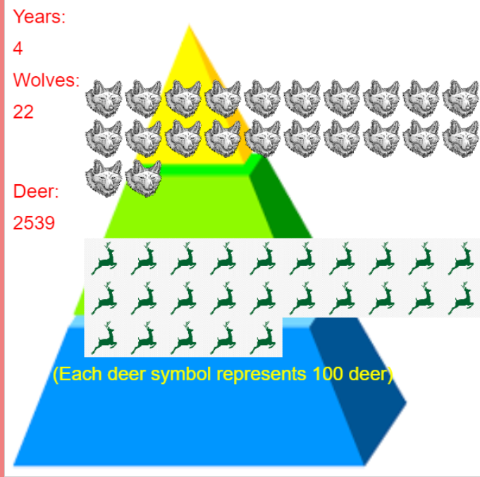
The exercise provides a simulation model of the introduction of predators into an environment. The model replicates a well studied classroom problem by implementing the growth rate equations of the predatpr and prey, predation rates, and the impact of environmental factors such as grass. After running the model with various inputs to learn its behavior, students can alter birth rates, starvation rates, and predation factors. The output is a graphcial representation of each population group, where each symbol represents a given number in that group.

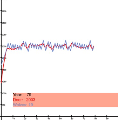
This exercise extends the previous predation model by displaying the oupput in a graphical form. Here students can watch the population move to equilibrium over time. The progression is not linear as each population group fluctuates over its peak during cosecutive time periods. The inputs and the model can be altered to measure the impact of increasing either population group or modifying the environment factor (grass).

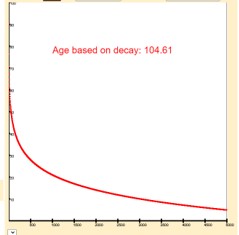
Carbon Decay rates are graphed in this exercise. Here the student can visualize utilizing radioactive isotopes and their half-life. In this activity the student will be calculating the age of a particular sample of carbon and then observing its decay graph. The model uses the common Carbon-14 relationship: N(t) = N₀ * e^(-λt). The student can adjust the initial value assignment and equations to calculate the amount remaining of a different radioactive isotope of their choice. The formulas are given as well as the repetitive call of the decay function which provides the data points for the graph. The worksheet prompts the student to make changes and record the impact.

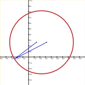
This science exercise focuses on orbits and their properties. Each planet's orbit is expressed with the focus of the sun and a focus of the planet. The exercises animate the path of the object in an orbit based upon particular ellipse around the foci and the associated eccentricity. Students are prompted with questions about the effect of changing the distance between foci and eccentricity. As the student makes changes, the animation illustrates the result of the new configuration.

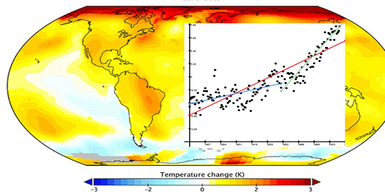
Climate change and global warming are the base topics for analysis in this exercise. Students can reference an instructor provided set of data (from a national weather source) about temperature change, mass variation, Artic ice, and sea levels. The model allows the student to tune the time frame and magnitude of the data to enable a clear trend to be identified on the graph. For example, students can calculate and visualize the slight weather changes from 1865 to 1957 versus the steep temperature increase since 1957. Students also see how the data must be processed and codified to some degree before the graphing process.

This exercise animates a ball of a specified mass falling from a student input height on one of 4 planets or the sun. The output includes some detailed statistics relating to gravity in these environments. Students are asked to do different simulations and then prompted for explanations of how the results differ by planet, mass and height. Key measurements include force , velocity , distance, and time. The animation done provides a more natural understanding of gravity in these different environments.

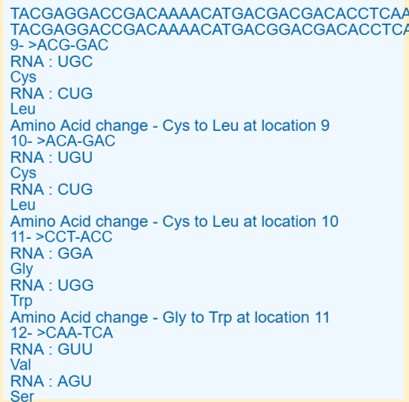
In this activity, the students will use the model to compare various strands of DNA to determine if the genetic mutation would cause albinism. Students will observe the normal genes that lead to melanin protein and compare each to three mutated sequences. By transcribing and translating each gene sequence in the model the student will determine both where the mutation is located and what type of mutation has occurred. The final steps determine how each gene was changed and how it affected the person’s phenotype. The model uses mappings of RNA to DNA codes as well as amino acid symbols.

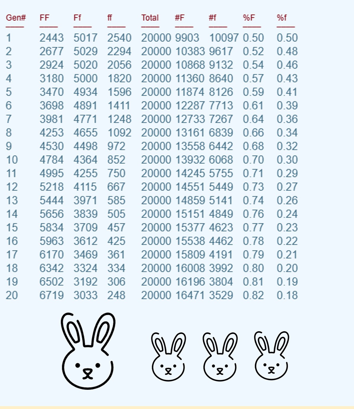
This topic examines natural selection in a small population of wild rabbits. The program code embeds the mathematical representation of the Hardy Weinberg model. Students can manipulate the survival rate and determine which traits are more advantageous. For example, if global warming continues, maybe having no fur is an advantage. This model enables the generation of various examples to be produced and analyzed. The exercise assumes the students have a strong understanding of Hardy Weinberg and genetic trait dominance combined with natural selection.

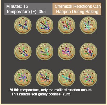
The model is a visualization using bar graphs to show how temperature impacts the reactions that occur during baking, starting from time 0 and ending at 15 minutes. Students can change the temperature of the baking process. Students can visually watch the cookies bake and see the impact of the chemical reaction of amino acids and reducing sugars. The goal is to find the best temperature and describe an overview of the chemical reactions.

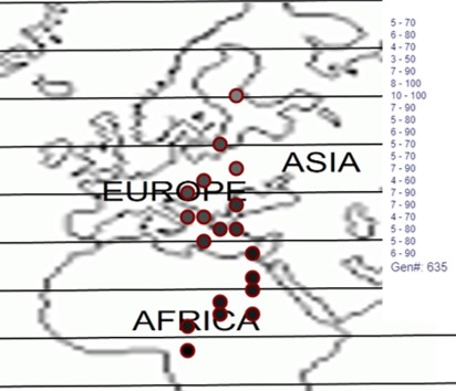
Variation in skin pigmentation was naturally selected based on latitude to balance protecting from harmful UV rays and allowing absorption of vitamin D. In this activity, students will observe the migration of Homo Sapiens over 100,000 years. Each generation in the model simulation will represent 1,000 years historically. The students will observe the melanin present (darkness of the circle) as the dot representations slowly migrate from Sub-Saharan Africa. Each student's simulation is random and can be recorded in the worksheet. The model tracks the population’s Melanin level as they migrate. The map is divided into Layers, similar to latitudes. Each layer has a level of Melanin that would maximize the survival rate, stored in LayerM. Each of the model’s 20 population groups starts at level 8 (middle Africa) with a Melanin level of 10. Population groups randomly migrate, and gain or lose Melanin randomly as well. Student can watch populations move over a world map through time.

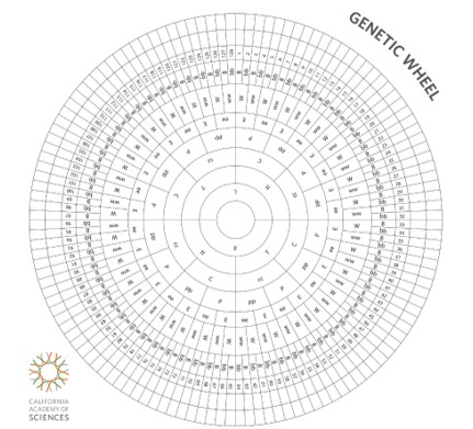
This exercise will introduce the students to dominant and recessive alleles and also map out the variation in single gene traits between themselves and their classmates using binary coding to come up with a unique variation number between 0-127. Having genetic variation within a species makes it more likely that some members of a population will survive under changing environmental conditions. Students can look around the room and notice the variations in size, hair color, eye color, etc. of classmates. The model prompts the students for specific trait questions. The answers are computed in a single sliver of the genetic wheel. Students can then compare their sliver locations to others in the class.

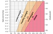
The Body Mass Index (BMI) value measures the healthy weight of a person based on their height and weight. The value produced relates to the tissue mass. This exercise produces a table for a person, showing their BMI for a healthy person. The table is geared for a particular height of a person. The ideal weights are then shown for a person of that height, according to BMI. BMI itself does not consider all factors that should be evaluated in determining obesity, and no categorization is mentioned in the exercise. Students can change the height shown by the table and compute BMI based on the height and weight of various inputs.